How and why do we attack our own Anti-Spam?

We often use machine-learning (ML) technologies to improve the quality of cybersecurity systems. But machine-learning models can be susceptible to attacks that aim to “fool” them into delivering erroneous results. This can lead to significant damage to both our company and our clients. Therefore, it is vital that we know about all potential vulnerabilities in our ML solutions and how to prevent attackers from exploiting them.
This article is about how we attacked our own DeepQuarantine ML technology, which is part of the Anti-Spam system, and what protection methods we deployed against such attacks. But first, let’s take a closer look at the technology itself.
DeepQuarantine
DeepQuarantine is a neural network model designed to detect and quarantine suspicious e-mails. It buys Anti-Spam system time to update our spam filters and do a rescan. The DeepQuarantine process is analogous to the work of an airport security service. Passengers who arouse suspicion are taken away for additional screening. The passenger has to wait while the security service inspects their baggage and checks their documents. If the all-clear is given, the passenger is allowed through, otherwise they are detained. In the case of the Anti-Spam system, the role of security service is played by Anti-Spam experts and services that process large flows of spam and create new detection rules while the e-mail is in quarantine; the role of the passenger’s baggage and documents goes to the e-mail headers. If the header analysis reveals new signs of spam messages, a detection rule is created based on the results. At the same time, other e-mails may be processed while the message is quarantined resulting in new detection rules. After the e-mail leaves quarantine, it is rescanned. If this triggers any of the new rules, the message gets blocked; if not, it is delivered to the recipient. Note that the quarantine technology needs to be very accurate so as not to delay legitimate e-mails — just as airport security cannot perform a full screening of every single passenger, as this would mess up the departure schedule.
Read more about how DeepQuarantine works here. To successfully attack an ML model, two things must be known: 1) what features it uses for decision-making; 2) how its training data is generated.
To identify suspicious e-mails, DeepQuarantine uses a sequence of technical headers (for example, the value of this feature in figure 1 would be “Subject:From:To:Date:Message-Id:Content-Type:X-Mailer”), plus the contents of the Message-Id (unique message identifier) and X-Mailer (mail client name) fields. These features were chosen because they depend on the type of mail client used and might contain traces of the spammer.

Figure 1. E-mail technical headers
Figure 2 illustrates how the algorithm operates. On the left is a real message from PayPal; on the right is a fake. For sending e-mails, the Message-Id is mandatory, and its format depends on the mail client. If we compare the headers of the fake with those of the original, what stands out is the lack of a domain and the random sequence of characters in this field.

Figure 2. Comparison of real and fake PayPal e-mail headers
These and other traces get left by scammers in various technical headers that the model processes and creating analytical rules to detect them is not a trivial task.
Now let’s look at the process of generating training data, which was the starting point for implementing the attack on our model.
Figure 3. Training sample generation scheme
Data and labels for training the model are generated automatically during general operation of the Anti-Spam system. The training sample generation scheme is shown in figure 3. After scanning messages, Anti-Spam forwards their headers and verdicts to Kaspersky Security Network (KSN), if the client has consented to data processing. From KSN, this data is sent to a repository, from where it is taken to train the model. Message headers are used as analysis samples, and verdicts from the Anti-Spam engine are used as labels.
Attacks on machine-learning models
What makes attacks on machine-learning models possible? Largely because, with machine-learning techniques, the distribution of data in the training sample is expected to match the distribution of data that the model encounters in the real world. Violation of this principle can lead to unexpected behavior on the part of the algorithm. Accordingly, attacks on machine-learning models can be divided into two kinds:
- Adversarial inputs — generating input data that causes an already trained and deployed model to deliver an incorrect verdict.
- Data poisoning — influencing the training sample to produce a biased model.
In the first case, in order to succeed, the adversary often needs to interact directly with the model. DeepQuarantine is only one component of the Anti-Spam system, so direct interaction with it is ruled out. The second type of attack is far more dangerous for our model. Let’s take a closer look.
Data-poisoning attacks can be further divided into two subtypes:
- Model skewing — contaminating the training sample in order to shift the model’s decision boundary. An example of such an attack is the targeting of Google’s spam classifier, in which advanced spam groups tried to contaminate the training sample by marking a large amount of spam as “not spam.” The aim was to make the system allow more spam messages through.
- Backdoor attack — introducing examples with a certain marker into the training sample to force an incorrect decision from the model, but only when this marker appears. For example, embedding a gray square in pictures belonging to a certain class (say, dogs), so that the model starts to recognize a dog when it sees this square. The picture might not be of a dog at all.
There are several ways to reduce the risk of a successful data-poisoning attack:
- Ensure that input data from a low number of sources (for example, from a small group of users or IP addresses) do not make up the majority of the training sample. This can make it harder for spammers to implement such attacks by forcing them to take additional steps to prevent their manipulations from being rejected as statistical outliers.
- Before releasing an updated version of the model, compare it with the latest stable version using a range of techniques such as A/B testing (comparing versions with various changes in a test environment), dark launch (running the updated service for a small pilot group of clients) or backtesting (testing the model on historical data).
- Create a benchmark dataset for which the correct evaluation result is known and against which you can validate the accuracy of the model.
Attack on DeepQuarantine
Now let’s move on to attacking DeepQuarantine. Let’s say the attacker’s goal is to have all e-mails sent by his employer’s rival company land in quarantine, which will badly impact its business processes. We investigate the attacker’s steps:
- Find out which mail client the company uses and what type of headers are generated when the company sends e-mails.
- Generate spam messages with headers similar to those of the victim company. Add some obvious spam-filter triggers to the body of the message, for example, explicit advertising or known phishing links, so that the messages are almost inevitably labeled as spam.
- Send these messages to our clients so that the Anti-Spam system blocks them and the related statistics get into the training and test sample, as illustrated in figure 3.
If, after being trained on the poisoned sample, the model passes testing, the attacked model is released, and e-mails from the victim company start being quarantined. Next, we experiment with different data-poisoning techniques.
Methodology
First, we took clean samples of training and test data, consisting of sets of e-mail headers with corresponding Anti-Spam verdicts. In both samples, we added poisoned headers mimicking the victim company with the verdict “spam” in varying amounts: 0.1, 1.5 and 10% of the sample size. For each experiment, the proportion of poisoned data in the training and test samples was the same.
Having trained the model on the poisoned training sample, we used the test sample to check the precision (proportion of correct positive verdicts out of all the model’s positive verdicts) and recall (proportion of correct positive verdicts out of the total number of spam headers in the sample) metrics, as well as the degree of confidence of “spam” verdicts assigned by the model to the victim company’s e-mails.
Experiment №1. Model skewing
Our first experiment implemented a model-skewing approach, as in the attack on Google’s anti-spam model. However, unlike the Google example, the aim was to simulate an attack on a specific company, which is a little more complicated. In this case, we used the domain of the chosen company (figure 4) in the Message-Id field, but the ID itself was generated randomly, retaining only the length specific to the mail client used by this company. We did not change the sequence of headers or the X-mailer field from the victim company’s mail client.

Figure 4. Poisoned example template
We analyzed how our target metrics (precision and recall) change on the test dataset depending on the proportion of poisoned data relative to the training sample size. The results are presented in figure 5. As seen in the graph, the target metrics remain almost unchanged relative to there being no poisoned examples in the data. This means that the model trained on the poisoned sample could be released.
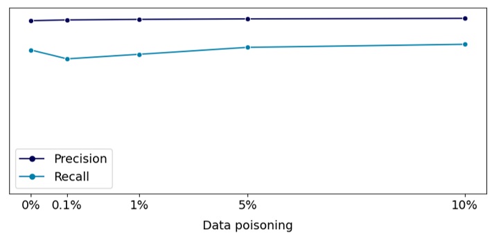
Figure 5. Target metrics depending on the amount of poisoned data
Using the headers of real e-mails from our chosen company, we additionally tested how data poisoning affects the model’s confidence that the message should be quarantined.
As illustrated in figure 5, when the share of poisoned data exceeds 5%, the model is already strongly inclined to believe that the victim company’s e-mails should be quarantined. Consequently, such a biased model could sever the correspondence between this company and our clients, which is what the attacker is trying to achieve.
|
|
|
|
|
|
|
|
|
|
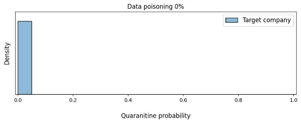


Figure 6. Change in the density of the model’s confidence in the need to quarantine the victim company’s e-mails based on the amount of data poisoning
Now, based on those objects that caused the model to make a wrong decision, let’s see what it was looking at. To do this, we built a series of Saliency Maps (see figure 6), using the Saliency via Occlusion method, in which the saliency of certain parts of the headers is established by alternately hiding these parts and assessing how this alters the confidence of the model. The darker the area in the picture, the more attention the neural network pays to this region in the decision-making process. The figure also shows how many e-mails from the chosen company (Target) and other companies (Other) land in quarantine.
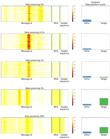
Figure 7. Saliency Maps
As we see in the graphs, as long as there is insufficient poisoned data for the model to return a false positive on e-mails from the victim company, the model concentrates mainly on the Message-Id field. But once the poisoned data becomes enough to bias the model, its attention becomes evenly distributed between Message-Id, the X-mailer field (MUA on the graph) and the sequence of headers in the e-mail (Header sequence).
Note that even though 5% poisoned data is enough for a successful attack, in absolute terms this is quite a lot of data. For example, if we use more than 100 million e-mails for training, an attacker would need to send more than 5 million, which would probably be picked up by the monitoring systems.
Can we attack our model more effectively? It turns out we can.
Experiment №2. Backdoor attack with timestamp
Some Mail User Agents specify timestamps in the Message-Id field. We used this fact to create poisoned headers with a timestamp corresponding to the model’s release date. In the event of a successful attack, the model quarantines e-mails from the victim company received on the day of release. Figure 8 shows how we generated the poisoned data.

Figure 8. Backdoor in data in the form of a timestamp
Does such data poisoning affect the target metrics in pre-release testing of the model? The result was the same as in the model-skewing attack (figure 9).

Figure 9. Target metrics depending on the amount of poisoned data
Was the attack more efficient in terms of the amount of data poisoning required? As we see in figure 10, the attacker in this case needed only 0.1% poisoned data to shift the model towards marking the victim company’s e-mails as suspicious.
|
|
|
|
|
|
|
|
|
|


Figure 10. Change in the density of the model’s confidence in the need to quarantine the victim company’s e-mails based on the amount of data poisoning
Let’s take a look at the Saliency Maps again to see what our model was paying attention to in this case. Figure 11 shows that at 0.1% poisoning, the model focuses on the domain start zone, agent type and header sequence. At 1% poisoning, the neural network mostly concentrates on the timestamp. We also notice that when the model is focused only on the timestamp, it issues more false positives on e-mails from other companies whose Message-Id also starts with a timestamp. As the level of poisoning increases, the model becomes focused on the timestamp and the domain start zone. At the same time, it shows no interest in the X-mailer field and the Header sequence.

Figure 11. Saliency Maps
Experiment №3. Backdoor attack with timestamp. Delayed attack
In the previous experiment, we were able to significantly improve the attack effectiveness. But in reality it is unlikely that an attacker would know the model release date. In this experiment, we decided to conduct a delayed attack to see if this would affect the test results. To do so, we generated poisoned headers with a timestamp shifted one year from the current release date (that is, not the same).
The results are shown in figure 12: the sample poisoning was not reflected in any way during testing, which is the most dangerous outcome for us, since it means an attack is almost impossible to detect. Given that the backdoor will be activated at an uncertain moment in the future, even dark launch and A/B testing will not help identify an attack.
|
|
|
|
|
|
|
|
|
|


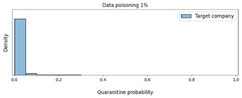


Figure 12. Dependence of the model’s confidence in the need to quarantine the victim company’s e-mails on the amount of data poisoning
From the results of the experiments, we drew the following conclusions:
- Model skewing requires a fairly large number of poisoned samples
- The fact of an attack is not reflected in precision and recall
- Adding a “backdoor” (in our case, a timestamp) makes the attack more effective
- Dark launch and A/B testing can be ineffective in the case of a delayed attack
We experimentally demonstrated a successful attack on our technology. But this prompts the question: how to defend against such attacks?
Protection against attacks on the ML model
In the context of our experiments, let’s take a closer look at ways to guard against data-poisoning attacks, which we mentioned in the “Attacks on machine-learning models” section: controlled selection of training data; techniques such as A/B testing, dark launch or backtesting; generation of a carefully controlled benchmark dataset. The controlled selection of objects for the training sample really does complicate attack implementation, because the attackers have to find a way to send fake data so that it is difficult to group and filter. This can be technically difficult, but, unfortunately, not impossible. For example, to prevent poisoned e-mails from being grouped by IP address, an attacker can use a botnet.
When it comes to creating an additional benchmark dataset that the model should fit very closely, in the case when the distribution of data changes over time, the question arises as to how long this dataset will remain current.
Comparing the updated model with the latest stable working version seems like a better solution, since this allows us to monitor changes in the models. But how to compare them with each other?
Let’s consider two options: comparing model versions on the current test dataset (Option 1), and comparing model versions on test datasets that are current at the time of release of each of the versions (Option 2). The table below shows the sequence of tests that we ran for both options.
| Option 1 | Option 2 |
| Comparison of quality metrics | Comparison of quality metrics |
| Tests for paired samples | Tests for independent samples |
| Homogeneity tests | Homogeneity tests |
First, we compared the target metrics of the models. At this stage we saw no significant variations between the original version and the updated one trained on a sample with varying degrees of data contamination. We obtained a similar result in the experimental attacks.
At the second stage of model comparison, we conducted a series of statistical tests:
- Student’s t-test on both paired and independent samples
- Wilcoxon signed-rank test on paired samples
- Mann–Whitney U test on independent samples
- Kolmogorov–Smirnov test for homogeneity of samples
The experiments revealed something curious: it turned out that the criteria produced significant differences even when comparing two models trained on a clean sample, although the predictive distributions of these models did not differ much from each other. This happened because, with a large amount of data, the tests are overly sensitive to the slightest changes in the shape of the distribution. But when we reduced the amount of data in the statistical tests, we often found no significant differences at all, because messages targeted in the attack might not even end up in the taken sample. Unsatisfied by this result, we developed our own criterion.
We proceeded from the fact that models trained on a clean sample differed little in terms of the distribution shape produced by the corresponding test datasets. While in the distribution of predictions of a model trained on a poisoned sample, “humps” can appear toward the right end of the distribution. Figure 13 shows one such large “hump” for illustrative purposes. In reality, though, it will be barely noticeable, since the volume of e-mails from the victim company will likely make up a small proportion of the total message flow.

Figure 13. Modeled distribution of model predictions on legitimate e-mails
In the course of the analysis, we arrived at the Wasserstein metric. In effect, this metric serves as a measure of the distance between distributions. Our criterion looks as follows:
H0: distributions of predictions on a sample of non-spam e-mails before and after training do not show statistically significant variations, that is, the system remained unchanged.
H1: variations in distributions are statistically significant, that is, the system has undergone changes.
We used the Wasserstein metric to assess the variations between the distributions of predictions of the old and new models on a sample of legitimate e-mails. To assess the statistical significance of the variations in the distribution of predictions, we needed to find out the distribution of these variations given a correct null hypothesis, that is, for versions of the model that did not undergo significant changes. We obtained this distribution using bootstrapping — sampling predictions of models trained on clean data, but in different time periods. In this way, we reconstructed the actual real-world situation. After that, we performed a series of statistical tests, comparing the distributions of the predictions of the original model and the model trained on a sample with different proportions of poisoned data. The Wasserstein criterion did not reveal significant differences for normal models, or for the model trained on delayed-attack data. This is to be expected, since we have seen that a delayed attack does not manifest itself in any way in the test. In other cases, however, we found significant differences. This means that the Wasserstein criterion allows us to detect most attacks of this kind in good time.
As for delayed attacks, and the general possibility of introducing a backdoor label into the data, a detailed data audit for potential backdoors is required. As is testing the machine-learning model for resistance to such attacks.
Takeaways
Ever more machine-learning methods are being introduced into various services. This raises performance indicators and improves the lives of users. However, it also makes new attack scenarios possible. Our experiment shows that:
- Data-poisoning attacks can do significant damage to machine-learning models.
- Attackers do not need to be data scientists.
- Timestamps can easily be used as a backdoor to attack a machine-learning model.
- Standard quality metrics do not reflect the fact of a data-poisoning attack.
- To reduce the likelihood of a successful attack on a model, the training and sampling process must be controlled.
- Extreme care must be taken when disclosing the details of model training and architecture so that attackers cannot exploit them.
- Before a model is released, the criteria used should be thoroughly tested to determine the model’s readiness and whether they can detect a potential attack. If the criteria are not sufficient to establish whether the model was attacked, it makes sense to develop your own.


